|
|
|
|
|
|
|
Using Equation 9.9, we get |
|
|
|
|
|
|
|
|
Note: a low population model (r = 5, n = 2) predicts ra = 0.32 and la = 16.2 (or 32.4 for two drives). |
|
|
|
|
|
|
|
|
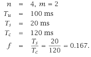
EXAMPLE 9.3 (m = 4, Ts = 20 MS) |
|
|
|
|
|
|
|
|
We now repeat Example 9.1 for m = 4 and Ts = 20 ms. |
|
|
|
|
| | | | | | | | | | | |
|
|
|
|
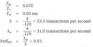
32.3 transactions per second |
|
|
|
| | | |
|
|
|
|
|
|
EXAMPLE 9.4 OTHER NOTES (n < 4, m ¹ 1) |
|
|
|
|
|
|
|
|
When n < 4 and m ¹ 1, we can model only with some error (see Figure 9.14). We know the result for n = 1, however. Regardless of m (the processor can use only one disk at a time), |
|
|
|
|
|
|
|
|
and there is no waiting time. |
|
|
|
|
|