
Previous Chapter Tutorial Home Next Chapter
Used with a utility like Ezmap or Conpack that creates lines dividing the plotter frame into regions, Areas allows you to retrieve (or recover) outline and other information about each region. Also, Areas allows you to overlay two or more groups or sets of lines, and to recover the regions defined by the union of the groups as well as telling you where each region is located relative to each group of lines. These features allow you to do things like mask contour lines or latitude/longitude lines over the ocean, and color-fill or pattern-fill regions.
The behavior of a typical routine in an NCAR Graphics utility is sometimes determined entirely by the routine's arguments, but frequently it is also affected by the value of one or more of the utility's "parameters." A parameter is a variable that controls the behavior of a utility; parameters are accessed via parameter-access routines that can set or retrieve the parameter value.
Instructions for setting and retrieving Areas parameters are provided in module "Ar 1.9 Areas parameters: What they do and how to use them."
-------------------------------------------------------------------
Parameter  Brief description         Fortran type  Examples  Module
-------------------------------------------------------------------
AT         Arithmetic Type flag      Integer
DB         DeBug plots flag          Integer       cardb1    Ar 4.1
DC         Debug Colors index        Integer
DI         Direction Indicator flag  Integer
LC         Largest Coordinate        Integer
-------------------------------------------------------------------
Three related concepts are very basic to Areas: edges, groups of edges, and group identifiers.
Figure 1 Figure 2
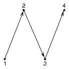
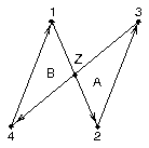
Figure 3 Figure 4
When one or more edges cross, Areas adds a vertex at each intersection so that regions such as A and B in Figure 2 can be addressed separately. When Figure 2 is drawn, it is defined by line segments (1,2), (2,3), (3,4), (4,1), but when the edges are processed by Areas, the point Z is added, and the edge segments defining the figure become (1,Z), (Z,2), (2,3), (3,Z), (Z,4), (4,1). These edge segments are among the building blocks of the Areas utility.
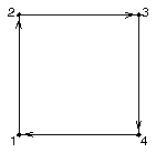
It is possible to define the same set of edge segments in many different ways. Looking at Figure 3, you can define the square as a single edge (1, 2, 3, 4, 1), or as two or more edges, like (1, 2, 3) and (3, 4, 1). In both cases, the square is defined by a set of edges: an edge group.
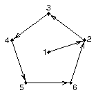
The most useful edge groups have no vertexes from which only one line segment emanates. In other words, useful edge groups won't have dangling line segments. This property implies that the plane is divided into discrete areas with well-defined boundaries. For example, the pentagon in Figure 4 divides the plotter frame into the area inside the pentagon and the area outside the pentagon. Notice that the line segment between points 1 and 2 in Figure 4 does have a vertex with precisely one line segment emanating from it. By default, Areas will remove dangling edges like this from the area map.
An area map is a linked list of edge segments, from which area and group information can be extracted. Area maps are discussed in module "Ar 1.6 Areas definitions: Areas, area identifiers, and area maps."
Ezmap produces dangling line segments. For instance, some small islands are crescent-shaped edges, so Areas will remove them from the area map.
Note: Areas definition modules Ar 1.3 through Ar 1.7 provide the background needed for the discussions in subsequent Areas modules. Because technically complete definitions involve complex mathematics that are not needed by most users, the definitions provided here are intended to give an intuitive understanding of the material.
Although you can assign any identifier to a specific group with Areas, it is helpful to know the group identifiers for the groups that are created with the Ezmap and/or Conpack utilities. The following group identifiers are the defaults used with Ezmap and Conpack:
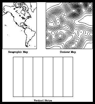
Using the graphic in this module, you could overlay the contour map over the geographic map; the map outlines would all be in group 1, and the contour lines would all be in group 3. By default, Ezmap produces a single vertical strip for the entire plot, so you would also have a group 2 defined that contains the perimeter of the geographic map. If you needed to overlay Conpack vertical strips as well, the Conpack vertical strips are placed in group 4 by default.
Note: Definitions in modules Ar 1.3 through Ar 1.7 provide the background needed for the discussions in subsequent Areas modules. Because technically complete definitions involve complex mathematics that are not needed by most users, the definitions provided here are intended to give an intuitive understanding of the material.
Figure 1a Figure 1b
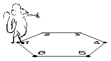
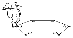
Figure 2 Figure 3
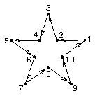
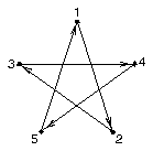
Figure 2 shows a more complex edge. In this case, the area inside the star is to the left of the edge, and the area outside the star is to the right of the edge. Figure 3 illustrates an edge that crosses itself. Areas breaks the edge down into edge segments, and then in sequential order, determines what is right of each edge segment and what is left of each edge segment. The preprocess area map modules Ar 2.3 through Ar 2.3.3 discuss how area information is reconciled for edges like the one in Figure 3.
Conpack always traces contour lines in such a way that the function being contoured slopes downhill to the left and uphill to the right. For this reason, areas where the function value is below the contour line are to the left and areas where the function value is above the contour line are to the right. Since this is always the case, we refer to areas above or below a contour line rather than to the left or right of a contour line.
Note: Definitions in modules Ar 1.3 -- Ar 1.7 offer an intuitive approach to understanding the material.
Figure 1 Figure 2a
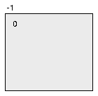
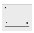
Figure 2b Figure 3a
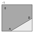
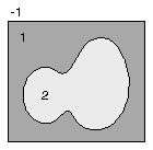
Figure 3b Figure 4

Let's look at some cases illustrating what this definition means. First, Areas defines a perimeter for the plotter frame so areas that would be otherwise unbounded can be identified and treated correctly by limited software and hardware. This perimeter is drawn around the limits of your plotter frame, but you can make any edge group inside your plotter frame into a perimeter. Figure 1 shows the default perimeter created by Areas.
First let's assume that we have two points, A and B, with an edge segment joining them. As shown in Figure 2a, the area defined by A and B is the entire plotter frame. When both A and B lie on different edges of the perimeter (Figure 2b), the edge segment (A, B) defines two areas, one to the left of the edge and one to the right of the edge.
A more complex case is that of a closed edge, or a loop (Figure 3a). In this case, what is outside the loop is an area, and what is inside the loop is an area. By adding one or more loops inside or outside the original, we now have areas within areas, or alternatively, holes within areas (Figure 3b).
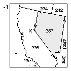
Another common edge group that defines areas is a set of intersecting edges, for example, a map of the US state boundaries. As shown in Figure 4, you can think of an area as a region that is defined by starting at an endpoint X on an edge segment, going to the end of that edge segment, choosing the leftmost connected edge segment, going to the end of it, choosing the leftmost connected segment, and so on, until you return the first edge segment (Figure 4). To define another area, start at an edge segment and choose only rightmost edges.
Each edge segment has a left area identifier and a right area identifier associated with it. As an area is defined, Areas keeps track of the area identifiers associated with each edge segment; if these don't all match, Areas decides which one has precedence. This process is discussed in detail in the preprocess area map modules 2.3 through 2.3.3.
Generally, negative area identifiers are all treated as if they were -1; this denotes areas outside the perimeter. Zero area identifiers are used to denote areas that have not yet had an area identifier assigned, or areas where you don't know what area identifier has been assigned by some other edge segment in the area map. Positive area identifiers should be used to denote any area that you may want to address. The numbers in the various areas in Figures 1 through 4 show possible area identifiers for each area.
An area map is a set of edge segments in the plane. There are three integers associated with each edge segment in the area map: a group identifier, a left area identifier, and a right area identifier. An area map is represented by a linked list of information that is constructed by calls to routines in the Areas utility. In the Fortran code, the area map (called MAP in the examples) is stored in a large integer array that is passed from subroutine to subroutine.
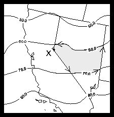
The previous module describes how to define an area by starting at an edge segment and tracing the leftmost edge segments until returning to the first edge segment. In that case, we traced out the state of Nevada as an area. In the lower figure, we overlay a contour edge group on the edge group defining the map of the western United States. Using the same approach as we used before, we now trace out the shaded area, the portion of a contour level over Nevada. Notice that as we do this, we choose the leftmost edge, regardless of which edge group it's in. In this case, the area has two area identifiers, one for the contour band that it's in and one for the state that it's in. As explained in module "Ar 1.4 Areas definitions: Groups of edges," contour levels are in edge group 3, and geographic maps are in edge group 1 by default.
The functional outline below shows how Areas works.
--------------------------------------------------------------
 *  1.  Open GKS
    2.  Set parameters
 *  3.  Initialize area map
 *  4.  Add edges to area map
 *  5.  Preprocess area map
 *  6.  Do one or more of the following:
 *      Break a polyline into segments, each of which lies
 entirely in a single area, then process each segment
 individually
 *      Retrieve area identifiers for areas containing a given
 point
 *      Scan an area map to retrieve each subarea, then
 process each subarea individually
    7.  Debug plot
 *  8.  Call FRAME
 *  9.  Close GKS
--------------------------------------------------------------
* Steps needed to produce a plot with Areas
The first argument in a call to ARGETI or ARSETI is the parameter name. The second argument is either a variable in which the value of the named parameter is to be returned (via ARGETI) or an expression specifying the desired new value of the parameter (via ARSETI).
CALL ARGETI (PNAM, IVAL)
CALL ARSETI (PNAM, IVAL)
Module "Ar 1.2 Table of Areas parameters" is a quick reference guide to all Areas parameters. Section "Ar 5. Areas parameter descriptions" provides more thorough descriptions of the Areas parameters.
Before you can use Areas, you must initialize an area map and add edges to it. Preprocessing area maps can then be done either directly or implicitly in the routines that produce results.
The last part of this section discusses preprocessing for users who want a deeper understanding of how Areas works.
--------------------------------------------------------------
    1.  Open GKS
    2.  Set parameters
 *  3.  Initialize area map
 *  4.  Add edges to area map
 *  5.  Preprocess area map
    6.  Do one or more of the following:
        Break a polyline into segments, each of which lies
 entirely in a single area, then process each segment
 individually
        Retrieve area identifiers for areas containing a given
 point
        Scan an area map to retrieve each subarea, then
 process each subarea individually
    7.  Debug plot
    8.  Call FRAME
    9.  Close GKS
--------------------------------------------------------------
* Steps discussed in this section.

1       CALL COLOR
2       CALL ARINAM (MAP, LMAP)
3       CALL AREDAM (MAP, XGEO, YGEO, NMAP, 1, 2, 1)
4       CALL AREDAM (MAP, XCNTR, YCNTR1, NPTS, 3, 2, 1)
5       CALL AREDAM (MAP, XCNTR, YCNTR2, NPTS, 3, 3, 2)
6       CALL AREDAM (MAP, XCNTR, YCNTR3, NPTS, 3, 4, 3)
7       CALL AREDAM (MAP, XCNTR, YCNTR4, NPTS, 3, 5, 4)
8       CALL AREDAM (MAP, XCNTR, YCNTR5, NPTS, 3, 6, 5)
CALL ARINAM (MAP, LMAP)
If you set the area map too small, the error message:
ERROR 5 IN AREDAM - AREA-MAP ARRAY
OVERFLOW
occurs when edges are added to the area map. There is no good way to predict exactly how large the area map should be before adding edges to it. Generally, if you are starting with a complex geographic map, start with an area map of 150,000 words. Most contour plots need between 50,000 and 100,000 words. Once you have your area map large enough, you can determine how much space was used by calculating:
MAP(1) - MAP(6) + MAP(5)where MAP is your area map after all the edges have been added to it. Areas routines ARPRAM and ARSCAM use more space during execution than after execution, so be sure to calculate your area map size after your last call to an Areas routine, and make your area map slightly larger than the calculated size.

1       CALL COLOR
2       CALL ARINAM (MAP, MAPSIZ)
3       CALL AREDAM (MAP, XGEO, YGEO, NMAP, 1, 2, 1)
4       CALL AREDAM (MAP, XCNTR, YCNTR1, NPTS, 3, 2, 1)
5       CALL AREDAM (MAP, XCNTR, YCNTR2, NPTS, 3, 3, 2)
6       CALL AREDAM (MAP, XCNTR, YCNTR3, NPTS, 3, 4, 3)
7
8       CALL AREDAM (MAP, XCNTR, YCNTR5, NPTS, 3, 6, 5)
 CALL AREDAM (MAP, XCURVE, YCURVE,
+ LCURVE, IGRP, IDLEFT, IDRGHT)
Line 4 adds the bottom contour line. It is drawn from left to right, and it is placed in group 3 in the area map just as Conpack does by default. The area to the right of each edge segment in this contour line is given an area identifier of 1, giving the bottom contour level an area identifier of 1. The area to the left of each edge segment in the first contour line is given area identifier 2. When the second contour line is added to the area map in line 5, it is also drawn from left to right, and it is added to group 3 in the area map. The area to the right of each edge segment in this contour line is also given area identifier 2. This gives the second contour band the same area identifier for both contours so that when the area map is reconciled, the second contour level will be given area identifier 2. Lines 6 through 8 add the rest of the contour lines in a similar fashion, giving each contour band a different area identifier.
Conpack uses much the same principle as this example. Each contour line in a contour plot is put in the same group. Then area identifiers for the area above and the area below the contour are assigned, given that Conpack always draws a contour so that the area below the contour line is to the left, and the area above the contour line is to the right. Each contour level is given a single area identifier, by default starting with 1 and going to n, where n is the number of contour levels in the plot.
If you count vertexes in each edge group, you can see that the number of vertexes nearly doubles when you put both edge groups in the same area map. By putting both vertexes in the same area map, you gain control over each sub-area. However, you also increase your area map size, and you increase the CPU time needed to process each area. Since Areas is one of the most CPU-intensive utilities in NCAR Graphics, this can significantly increase the time needed to run your program. In many cases, you can produce results significantly faster by putting your geographic outlines in one area map, your contour lines in another area map, then using masking.
Frame 1 Frame 2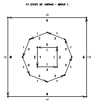
Frame 3 Frame 4
CALL ARPRAM (MAP, IF1, IF2, IF3)
Step 1: ARPRAM shortens edge segments whose projections on the X axis are more than twice as long as the average. ARPRAM does this by interpolating points along their lengths. This improves efficiency when executing other parts of the algorithm.
Step 2: ARPRAM locates all intersections of edge segments and interpolates the intersection points along these edge segments. This step can take a lot of time. If you set IF1<>0, then pairs of edge segments are examined for intersections only if one of the pair has a left or a right area identifier that is zero or negative.
Step 3: ARPRAM removes coincident edge segments (those with identical endpoints). If two coincident edge segments belong to the same group, one of them is removed; if they belong to different groups, one of them is modified in such a way that it will appear to be present when looking for areas defined by edge segments in a particular group, but absent when looking for areas defined by all edge segments.
Step 4: ARPRAM searches for and removes "dangling" edges (those that do not contribute to enclosing any area). This step is skipped if IF2<>0.
Step 5: ARPRAM looks for holes in the areas defined by each edge group and draws connecting edge segments between the edge and the hole. This step is skipped if IF3<>0.
Step 6: ARPRAM adjusts area identifier information in the area map. It examines all the edge segments of each area in each group to see what area identifier should be assigned to the area, and then makes adjustments.
Step 7: Connecting lines that were inserted in step 5 are removed from the area map.
You can put edges in an area map, preprocess it, add more edges, preprocess it again, and so on.
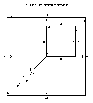
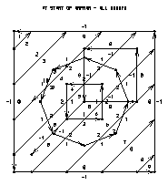
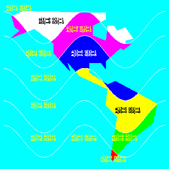
No discussion is given about the code that generates plots for the four modules in this preprocess area map group. Rather than analyzing the code, study the plots to learn how ARPRAM operates. Frames 1 through 3 from this code show the three edge groups that are added to the area map before processing, and frame 4 shows the entire area map before processing. The arrows show the direction of each edge segment, and the small numbers on each side of each edge segment are the left and right area identifiers for the segment.
Frame 1  Frame 5

Frame 8  Frame 12
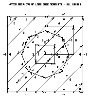
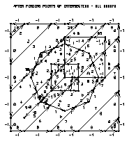
Step 2 breaks up edge segments at points of intersection with other edge segments. Compare frames 8 and 12; notice how Areas adds a vertex wherever an edge segment meets another edge segment, regardless of which groups the edge segments are in. It also shows that both edge segments are divided into shorter edge segments at that vertex.
More precisely, ARPRAM decides where to break edge segments if an edge segment (P,Q) is crossed by another edge segment at point I, where I is distinct from P and Q. ARPRAM then breaks (P,Q) into two edge segments, (P,I) and (I,Q). Clearly, this process can considerably increase the size of the area map. Also note that ARPRAM finds these points of intersection regardless of which group or groups the affected edge segments are in. Frame 12 shows the area map after this step is completed.
As discussed in the previous module, step 2 can be abbreviated by calling ARPRAM with IF1<>0. In this case, edge segments are examined for intersection only if one of the pair has a right or a left area identifier that is zero or negative. This is appropriate for contour lines, or if you know that you have equally "nice" edges that don't cross anywhere except at the perimeter.
Frame 10 Frame 14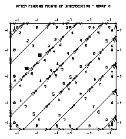
Frame 11 Frame 19
This step ensures that areas are correctly traced when tracing an area boundary using the method of following rightmost or leftmost edge segments.
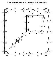
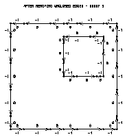
Step 4 removes dangling edge segments (edge segments that do not contribute to forming any areas). A dangling edge is any edge that has an endpoint with only one edge segment in an edge group emanating from it. Examples of dangling edges include a single line segment with endpoints not on the perimeter, short curves drawn by Ezmap to represent islands, and in frame 11, the tail on the square. Note that the tail is drawn as part of group 5; however, after step 4 is done for frame 19, the tail has been removed from the area map.
Frame 17 Frame 21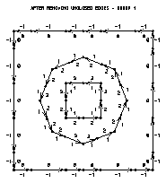
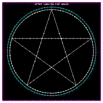
Simplified figure Frame 25
Holes are important because an area with a hole does not have a boundary that is a simple closed curve. Instead, the boundary consists of two or more simple closed curves; one of these forms the outer boundary of the area and the others form the holes. This complicates things for Areas because, in attempting to reconcile contradictory area identifier information, it can only look at one closed curve at a time; contradictory information on two different parts of the boundary of an area with holes would therefore not be reconciled.
In step 5, ARPRAM identifies holes and adds temporary edge segments to the area map to, in effect, remove the holes. These edge segments ensure that all the areas in the area map have boundaries that are simple closed curves. Thus, as ARPRAM traces the boundary of one area, it sees all of the area identifiers that have been provided by the user for that area.
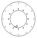
Frames 17 and 21 show edge group 1 before and after step 5. Consider the area having the perimeter as an outer boundary and the octagon as a hole. Information provided with the perimeter says that its area identifier should be 0, but information provided with the octagon says that its area identifier should be 1. Step 5 inserts a vertical connecting line between the perimeter and the octagon, making it possible to trace the boundary of the area as a single simple closed curve, so that all area-identifier information can be considered at once and the contradiction can be seen and reconciled.
ARPRAM methodically traces all the area boundaries defined by an area map: it repeatedly selects an edge segment to start with and makes either leftmost turns only or rightmost turns only until it arrives back at the starting point. Edge segments seen while doing this are marked so that a given boundary is only traced once.
Holes are detected by keeping track of the total change in direction along each boundary as it is traced. Net changes in angular direction to the right (clockwise) are considered negative, and net changes in angular direction to the left (counterclockwise) are considered positive. The net change along a boundary will always be exactly +360 or -360 degrees. Either of the following two cases is sufficient to confirm the existence of a hole:
If you set IF3 nonzero, ARPRAM will not look for holes. This should only be done when you can be absolutely sure that area identifier information for holes in an area does not contradict that for the outer boundary of the area.
In step 6, ARPRAM again traces all of the boundaries in the area map. This time, ARPRAM assumes that each such boundary defines precisely one area, and it reconciles the area identifier information given for that area with the edge segments defining that boundary. After ARPRAM has picked an area identifier for the area, it replaces all the area identifiers for those edge segments with the value selected. If any of the area identifiers examined is negative, a -1 will be used; if all of the area identifiers examined are zeroes, a 0 will be used; otherwise, the nonzero value most recently entered in the area map will be used.
In step 7, ARPRAM removes the temporary edge segments that were added in step 5.
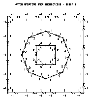
In frame 25, note that the temporary edge segments added in step 5 have been removed and that the area identifiers on the inside of the perimeter now match the values on the outside of the octagon.
--------------------------------------------------------------
    1.  Open GKS
    2.  Set parameters
    3.  Initialize area map
    4.  Add edges to area map
    5.  Preprocess area map
 *  6.  Do one or more of the following:
 *      Break a polyline into segments, each of which lies
 entirely in a single area, then process each segment
 individually
 *      Retrieve area identifiers for areas containing a given
 point
 *      Scan an area map to retrieve each subarea, then
 process each subarea individually
    7.  Debug plot
    8.  Call FRAME
    9.  Close GKS
--------------------------------------------------------------
* Steps discussed in this section.
1       DO 20, I=1, 12
2          CALL ARGTAI (MAP, X(I), Y(I), IAREA, IGRP, NGRPS, NAI, 0)
3          DO 30, J=1, 2
4                 WRITE (STRING, 11) J, IAREA(J), J, IGRP(J)
5                 IF (IGRP(J) .EQ. 1) THEN
6                        CALL GSPLCI(1)
7                        CALL PLCHHQ (X(I), Y(I), STRING, .01, 0., 0.)
8                 ENDIF
9                 IF (IGRP(J) .EQ. 3) THEN
10                       CALL GSPLCI(6)
11                       CALL PLCHHQ (X(I), Y(I) -.018, STRING, .01, 0., 0.)
12                ENDIF
13 30          CONTINUE
14 20   CONTINUE
 CALL ARGTAI (MAP, XCD, YCD, IAREA,
+ IGRP, ISIZ, NGRPS, ICF)
ARGTAI has also been used to determine whether a specific point is over land or water. A user created a fine grid over the globe and used ARGTAI to determine if each point in the grid was over land or water. Then he used the resulting array to tell his model which points were over land and which points were over water.

1       EXTERNAL MASK
2       CALL ARINAM (MAP, LMAP)
3       CALL AREDAM (MAP, XGEO, YGEO, NGEO, 1, 2, 1)
4       CALL ARDRLN (MAP, XCNTR, YCNTR1, NPTS, XWRK, YWRK, NWRK,
       + IAREA, IGRP, NGRPS, MASK)
5       CALL ARDRLN (MAP, XCNTR, YCNTR2, NPTS, XWRK, YWRK, NWRK,
       + IAREA, IGRP, NGRPS, MASK)
6       CALL ARDRLN (MAP, XCNTR, YCNTR3, NPTS, XWRK, YWRK, NWRK,
       + IAREA, IGRP, NGRPS, MASK)
7       CALL ARDRLN (MAP, XCNTR, YCNTR4, NPTS, XWRK, YWRK, NWRK,
       + IAREA, IGRP, NGRPS, MASK)
8       CALL ARDRLN (MAP, XCNTR, YCNTR5, NPTS, XWRK, YWRK, NWRK,
       + IAREA, IGRP, NGRPS, MASK)
 CALL ARDRLN (MAP, XCD, YCD, NCD,XCS,
+ YCS, MCS, IAREA, IGRP, ISIZ, LPR)
Before executing the first call to LPR, ARDRLN calls GETSET to retrieve the current user-system mapping parameters, then executes the statement:
 CALL SET (VPL, VPR, VPB, VPT, VPL,
+ VPR, VPB, VPT, 1)
where VPL, VPR, VPB, and VPT are the viewport left, right, bottom, and top coordinates in NDCs.
This ensures correct results if the NDCs in XCS and YCS are used in calls to such routines as GPL and CURVE, and this allows clipping at the edges of the viewport. LPR may make its own SET call to achieve some other effect. Before returning control to the calling routine, ARDRLN calls SET again to restore the original mapping parameters.
In the carline example, XGEO and YGEO are arrays containing the X and Y coordinate information for the "geographical" outline. XCNTR and YCNTR1-4 are the X and Y coordinate arrays for the "contour" lines. Line 1 declares our masking routine to be external so that Fortran doesn't interpret the subroutine name as a variable. Line 2 initializes Areas. Line 3 adds the geographic outline to the area map in group 1 for consistency with Ezmap defaults. Lines 4 through 8 show examples of calling ARDRLN to mask the contour lines over land masses, where MASK is the actual line-drawing and masking routine.
When drawing lines with ARDRLN, it is best not to add the lines to the area map.

1       SUBROUTINE MASK (XC, YC, MCS, IAREA, IGRP, NGRPS)
2       INTEGER IAREA(NGRPS), IGRP(NGRPS), IDGEO
3       REAL XC(MCS), YC(MCS)
4       IDGEO = -1
5       DO 10, I=1, NGRPS
6          IF (IGRP(I) .EQ. 1) IDGEO = IAREA(I)
7   10  CONTINUE
8       IF (IDGEO .EQ. 1) THEN
9          CALL CURVED (XC, YC, MCS)
10      ENDIF
11      RETURN
12      END
 SUBROUTINE LPR (XCS, YCS, NCS,
+ IAREA, IGRP, ISIZ)
 DIMENSION XCS(*), YCS(*), IAREA(*),
+ IGRP(*)
 SUBROUTINE LPR (XCS, YCS, NCS,
+ IAREA, IGRP, ISIZ)
 DIMENSION XCS(*), YCS(*), IAREA(*),
+ IGRP(*)
RETURN
END

1       EXTERNAL FILL
2       CALL GSFAIS (1)
3       CALL ARINAM (MAP, LMAP)
4       CALL AREDAM (MAP, XGEO, YGEO, NMAP, 1, 2, 1)
5       CALL AREDAM (MAP, XCNTR, YCNTR1, NPTS, 3, 2, 1)
6       CALL AREDAM (MAP, XCNTR, YCNTR2, NPTS, 3, 3, 2)
7       CALL AREDAM (MAP, XCNTR, YCNTR3, NPTS, 3, 4, 3)
8       CALL AREDAM (MAP, XCNTR, YCNTR4, NPTS, 3, 5, 4)
9       CALL AREDAM (MAP, XCNTR, YCNTR5, NPTS, 3, 6, 5)
10      CALL ARSCAM (MAP, XWRK, YWRK, NWRK, IAREA, IGRP, NGRPS, FILL)
 CALL ARSCAM (MAP, XCS, YCS, MCS,
+ IAREA, IGRP, ISIZ, APR)
All regions having the same group and area identifiers are treated the same way. In this example, every separate piece of a single contour band over land is filled with the same color. This is why the color of western Alaska matches the color of central Canada. If you want to color a contour over Canada differently than the same contour over the US, you would have to add the political boundaries to your area map, then give Canada a different area identifier than the US. Fortunately, Ezmap can do this for you.
Line 1 of the carfill.f code segment declares our filling routine FILL to be external so that when we call it, Fortran doesn't interpret the subroutine name as a variable and then core dump. Line 2 sets the GKS fill style to be solid because the default is "hollow" fill. Line 3 initializes Areas. Lines 4 through 9 add "geographic" and "contour" lines to the area map using group 1 for geographic outlines and group 3 for contour lines; this ensures consistency with Conpack and Ezmap defaults. Line 10 does the area fill by calling ARSCAM, which examines the area map and feeds the appropriate information to the fill routine FILL. The next module describes the FILL routine.
1       SUBROUTINE FILL (XWRK, YWRK, NWRK, IAREA, IGRP, NGRPS)
2       INTEGER IAREA(NGRPS), IGRP(NGRPS), IDGEO, IDCNTR
3       REAL XWRK(NWRK), YWRK(NWRK)
4       IDGEO = -1
5       IDCNTR = -1
6       DO 10, I=1, NGRPS
7          IF (IGRP(I) .EQ. 1) IDGEO = IAREA(I)
8          IF (IGRP(I) .EQ. 3) IDCNTR = IAREA(I)
9   10  CONTINUE
10      IF (IDGEO .EQ. 1) THEN
11         CALL GSFACI(7)
12         CALL GFA (NWRK, XWRK, YWRK)
13      ELSE IF ((IDGEO .EQ. 2) .AND. (IDCNTR .GE. 1)) THEN
14         CALL GSFACI(IDCNTR)
15         CALL GFA (NWRK, XWRK, YWRK)
16      ENDIF
17      RETURN
18      END
 SUBROUTINE APR (XCS, YCS, NCS,
+ IAREA, IGRP, ISIZ)
 DIMENSION XCS(*), YCS(*), IAREA(*),
+ IGRP(*)
 SUBROUTINE APR (XCS, YCS, NCS,
+ IAREA, IGRP, ISIZ)
 DIMENSION XCS(*), YCS(*), IAREA(*),
+ IGRP(*)
RETURN
END
After the area identifiers have been obtained, line 10 checks to see if we're over the ocean. If we are, then lines 11 and 12 fill the area in aquamarine. Line 13 checks to see if we're over land, and if so, then lines 14 and 15 fill the contour band with a color based on its area identifier.
APR can be used to do almost anything you want with each area in the area map. However, it is rarely used for anything except filling areas. If you are unable to produce color hardcopy output, you may want to write your fill routine so that it calls the Softfill utility.
Before executing the first call to APR, ARSCAM executes the statement:
 CALL SET (VPL, VPR, VPB, VPT, VPL,
+ VPR, VPB, VPT, 1)
where VPL, VPR, VPB, and VPT are the viewport left, right, bottom, and top coordinates in NDCs. This ensures correct results if the NDCs in XCS and YCS are used in calls to such routines as GFA and FILL, and this allows clipping at the edges of the viewport. APR may make its own SET call to achieve some other effect. Before returning control to the calling routine, ARSCAM calls SET again to restore the original mapping parameters.
--------------------------------------------------------------
    1.  Open GKS
 *  2.  Set parameters
    3.  Initialize area map
    4.  Add edges to area map
    5.  Preprocess area map
    6.  Do one or more of the following:
        Break a polyline into segments, each of which lies
 entirely in a single area, then process each segment
 individually
        Retrieve area identifiers for areas containing a given
 point
        Scan an area map to retrieve each subarea, then
 process each subarea individually
 *  7.  Debug plot
    8.  Call FRAME
    9.  Close GKS
--------------------------------------------------------------
* Steps discussed in this section.
1       CALL ARINAM (MAP, MAPSIZ)
2       CALL ARSETI ('DB - DEBUG PLOTS FLAG', 1)
3       CALL AREDAM (MAP, X1, Y1, NPTS, 1, 1, 0)
4       CALL AREDAM (MAP, X2, Y2, NPTS, 1, 2, 1)
5       CALL AREDAM (MAP, X3, Y3, NVERT, 1, 3, 2)
6       CALL ARSCAM (MAP, XC, YC, MCS, AREAID, GRPID, IDSIZE, FILL)
CALL ARSETI ('DB', idb)
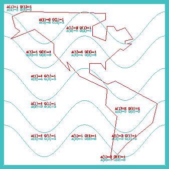
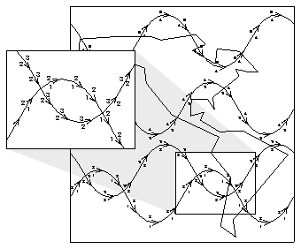
In each of the debug plots, notice the dots on each side of each line segment. These are numbers that represent the left and right area identifiers for that edge. To view them, you need to use the zoom feature in idt.
The area identifiers are drawn very small so that each edge segment in an area map can be marked with both left and right area identifiers.
1       CALL ARINAM (MAP, LMAP)
2       CALL AREDAM (MAP, XGEO, YGEO, NMAP, 1, 2, 1)
3       CALL AREDAM (MAP, XCNTR, YCNTR1, NPTS, 3, 2, 1)
4       CALL AREDAM (MAP, XCNTR, YCNTR2, NPTS, 3, 3, 2)
5       CALL AREDAM (MAP, XCNTR, YCNTR3, NPTS, 3, 4, 3)
6       CALL AREDAM (MAP, XCNTR, YCNTR4, NPTS, 3, 5, 4)
7       CALL AREDAM (MAP, XCNTR, YCNTR5, NPTS, 3, 6, 5)
8       CALL ARDBPA (MAP, 3, 'Crossing Contours')
CALL ARDBPA (MAP, IGRP, LABEL)
In the zoomed portion of the picture, notice how the left and right area identifiers are in conflict in the areas above and below the crossed contour lines. This situation occasionally arises when using smoothing in Conpack. When Areas is used in a situation like this, the contour bands may be filled in an undesired fashion, since the areas do not have well-defined identifiers.
By default, each edge in the plot appears in one of four different colors, depending on whether the area identifiers to the left and right are less than or equal to zero or greater than zero, as follows:
--------------------------------
Color    Left area   Right area
         identifier  identifier
--------------------------------
Magenta  <=0      <=0
Yellow   <=0      >0
Cyan     >0       <=0
White    >0       >0
--------------------------------
You can adjust these colors with the DC parameter.In some cases, you may notice gray lines in your plot. This means that the same edge occurs in more than one group. In all but one of those groups, Areas negates the group identifier for the edge in the area map. This allows Areas to include the edge when it is looking at a particular group (as in ARPRAM), but omit it when it is looking at the union of all the groups (as in ARSCAM).
If ARDBPA is used for a complicated area map, the amount of output can be very large.
Previous Chapter Tutorial Home Next Chapter