|
|
|
|
|
|
|
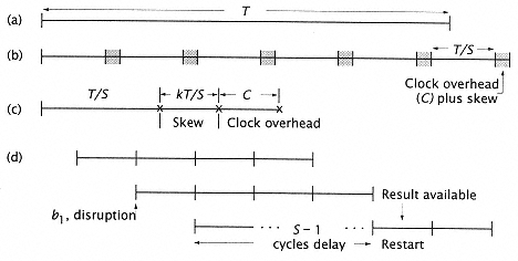
Figure 2.10
Optimal pipelining. (a) Unclocked instruction execution time, T. (b) T is
partitioned into S segments. Each segment requires C + (k)t/s clocking
overhead and skew. (c) Clocking overhead and its effect on cycle time T/S.
(d) Effect of a pipeline disruption (or a stall in the pipeline). |
|
|
|
|
|
|
|
|
processor. Our analysis is based on the work of Kunkel and Smith [175] and Dubey and Flynn [77]. |
|
|
|
|
|
|
|
|
Assume that the total time to execute an instruction without latches or pipeline segments is T nanoseconds (Figure 2.10a). Now T is to be segmented into S segments to allow clocking and pipelining. The ideal delay through a segment is T/S = Tseg. Associated with each segment are two types of partitioning overhead: |
|
|
|
|
|
|
|
|
1. A fixed clock overhead time C (in ns), including data setup and hold. |
|
|
|
|
|
|
|
|
2. A variable linear ''stretching" factor k that increases the segment delay (T/s) by a factor of (1 + k). Assume 0 < k < 1. This accounts for such effects as clock skew (Figure 2.10b). As cycles (T/s) get larger, more complex functions are incorporated into the cycle. This increases clock distribution difficulties and hence clock skew. |
|
|
|
|
|
|
|
|
Therefore, the actual cycle time (Figure 2.10c) of the pipelined processor is the ideal cycle time T/S plus the overhead: |
|
|
|
|
|
|
|
|
Now consider our idealized pipelined processor. If there are no code interruptions, it processes instructions at the rate of one per cycle; but interruptions can occur (primarily due to incorrectly guessed or unexpected branches, as we shall see in more detail in Chapter 4). Suppose these interruptions occur with frequency b and have the effect of invalidating the S - 1 instructions prepared to enter, or already in, the pipeline (representing a "worst-case" disruption, Figure 2.10d). As we shall see in Chapter 4, there are many different types of pipeline interruption, each with a different effect, but this simple model illustrates the effect of disruptions on performance. |
|
|
|
|
|