|
|
|
|
|
|
|
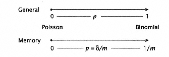
Figure 6.15
Characterizing request distributions with p.
For the memory model, n items enter the
system (or request), each with probability d. |
|
|
|
|
|
|
|
|
There is still another modeling possibility. Suppose we have the relationship described in Figure 6.14, but the probability of a request in any particular processor cycle is nonzero, say p = d. In the context of m interleaved memory modules, this means that the probability of a request to a particular module is  . In memory systems, we will refer to the case wherein the request sources (or items that enter the system) request or enter with probability d as the d-binomial distribution. (See Figure 6.15.) . In memory systems, we will refer to the case wherein the request sources (or items that enter the system) request or enter with probability d as the d-binomial distribution. (See Figure 6.15.) |
|
|
|
|
|
|
|
|
6.4.3 Service Distribution |
|
|
|
|
|
|
|
|
From a service point of view, there are three Markovian (i.e., memoryless) distributions of particular interest. |
|
|
|
 |
|
|
|
|
All requests take time T for service,  |
|
|
|
|
|
|
|
|
Exponential Service-Time Distribution |
|
|
|
|
|
|
|
|
The probability that service is completed by time t (m is average service rate) is |
|
|
|
|
|
|
|
|
P(t) = 1 - e-mt. |
|
|
|
|
|
|
|
|
The distribution for the time (t) between arrivals in a Poisson distribution is the exponential distribution. This can be seen by assuming the time of last arrival at a server is 0 and the time of a current arrival is a random variable t. Then the distribution of Poisson arrival times is |
|
|
|
|
|
|
|
|
Prob (time between arrivals is < t) |
|
|
|
|
|
|
|
|
= 1 - Prob (time between arrivals is t). |
|
|
|
|
|
|
|
|
This latter probability is simply the probability of no arrivals between 0 and t (i.e., k = 0 in the Poisson distribution). Thus, |
|
|
|
|
|
|
|
|
Prob (time between arrivals is <t) = 1 - e-lt, |
|
|
|
|
|
|
|
|
where 1 / l is the mean of the interarrival time distribution. So if 1/m is the mean interservice time, then the interservice probability is |
|
|
|
|
|
|
|
|
P(t) =1 - e-mt. |
|
|
|
|
|