|
|
|
|
|
|
|
|
Prob[no processor references the module] |
|
|
|
| | | | | | | | | |
|
|
|
|
B(m,n) = average number of busy modules |
|
|
|
| | |
|
|
|
|
|
|
The achieved memory bandwidth is less than the theoretical maximum due to contention. By neglecting the congestion that has carried over from previous cycles, this analysis results in an optimistic value for the bandwidth. Also, as in the previous example, the two modeling assumptions cause the calculated bandwidth to be higher still. |
|
|
|
|
|
|
|
|
It has been shown by Bhandarkar [35] that B(m, n) is almost perfectly symmetrical in m and n. He exploited this fact to develop a more accurate expression for B(m, n), which is |
|
|
|
|
|
|
|
|
where K = max(m, n) and l = min (m, n). |
|
|
|
|
|
|
|
|
The most accurate closed-form solution for B(m, n) for multiple simple processors is based upon the work of Rau [241], and is based upon the following analytic approximation. |
|
|
|
|
|
|
|
|
All processors not awaiting service at a given memory module are queued at the remaining m - 1 modules with precisely the same distribution that would occur in a system consisting of the same number of processors and m - 1 memory modules. |
|
|
|
|
|
|
|
|
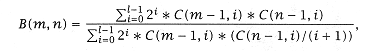
The result of an analysis based on this approximation is that Closed form: |
|
|
|
|
|
|
|
|
where C(x, y) is the number of ways of choosing y objects out of a set of x objects, and l = min (m, n). When compared with the exact results from a Markov chain analysis [35] (see shortly), the preceding expression is never more than 0.25% in error, attesting to the accuracy of the analytical approximation. |
|
|
|
|
|
|
|
|
These results are compared in Tables 6.1 and 6.2. |
|
|
|
|
|
|
|
|
6.4 Processor-Memory Modeling Using Queueing Theory |
|
|
|
|
|
|
|
|
Simple processors are unbuffered; when a response is delayed due to a conflict this delay directly affects processor performance by the same amount. |
|
|
|
|
|